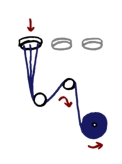
Supply chain planning for a manufacturer of polyester yarn.  Molten polyester (PET) is extruded through a "spinneret" (something like a shower head) to produce multiple strands – up to 300.  The strands from one spinneret are cooled, oiled, rolled, stretched and twisted together to form a single filament, which is wound onto a reel.  The product grade is determined by the choice of spinneret (number of holes and diameter), the temperature and flow rate, and additives in the PET.

Spinnerets are normally grouped into 6, 8 or 12 in one "position" and all the spinnerets in one position make the same product.  Positions are grouped into "housings" and housings into "groups", and finally a production line is normally made up of two groups.  In total, there are normally 36 positions in a production line.  In this application, there are over 30 spinning lines.

Each line has a subset of products that it is able to make, and preferences based on quality within that subset.  Changeovers involving a change of spinneret are expensive, because of the time taken to refit, and because the spinnerets cannot be reused once removed.  (The metal is recycled.)

Most of the lines are capable of making multiple products at one time, though there is a practical limit of three products at once.  There are complex restrictions on which products can run together, arising from feasible temperature and flow rate bands, which are controlled at different levels in the equipment hierarchy.

Modelling these restrictions is too complex to discuss here.  A more fundamental question is how to model spinneret changeovers without having to model individual positions.

If we do not model the changeovers, the cost cannot be recognised, and the optimal solution may contain an unacceptable variability of products on some lines.  If we model individual positions, we get a huge number of zero-one variables representing the decision to make each product at each position in each time period (weeks and months), and the model becomes impossible to solve.

That is not the end of the problems – standard changeover modelling simply counts the number of products in each period and ignores the benefit of continuing to make the same product over the time period end.  (This is because you then need to be concerned about which product is first and last in each period, which adds a level of complexity.)

We use an extra piece of information.  Changeovers are such a large part of the cost that most of the time a position will run the same product for at least a time period and often more than one.  This makes it (just about) reasonable to assume that changeovers will only happen at period ends.  Instead of assigning products to individual positions, we can just calculate the number of positions needed to make the planned quantity over the time available.

Production rate and period length are constants, so this is a linear relationship between quantity of product and number of positions.  Number of positions is defined as a continuous variable, so two and a half positions is possible.  This is nonsensical, but forcing the variable to take integer values would over-restrict the possible production levels.

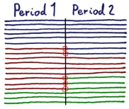
We need to derive the number of changeovers.  Suppose 6 positions make product 1 in the first period, and 8 positions make product 1 in the next.  Then at the very least, two positions must change over from whatever they were making in the first period at the start of the next.  This is just a linear constraint:

We apply the changeover costs to this minimum value and accumulate over all products.  The net result is that we have a fairly inaccurate but very computationally cheap measure of the total cost of changeovers.  We should not expect to be more accurate in a model with long time periods.  More important than accuracy, we can now penalise changes in product mix on each line over time, so steady production is encouraged.  The optimal solution provides a good starting point for detailed daily scheduling.